Elastic Distances¶

Distance measures that perform a non-linear mapping to align the time series and allow flexible comparison of one-to-many or one-to-none points (e.g., Dynamic Time Warping, Longest Common Subsequence). These measures produce elastic adjustment to compensate for potential localized misalignment.

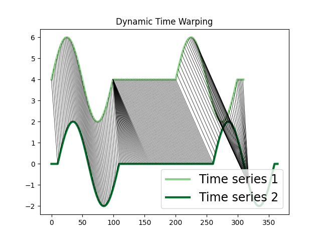
Dynamic Time Warping (DTW)¶

The DTW algorithm computes the stretch of the time axis which optimally maps between two time series. It measures the remaining cumulative distance after the alignment and the pairwise correspondence between each sample.

import numpy as np
import matplotlib.pyplot as plt
from tssearch.search.query_search import time_series_search
from tssearch.utils.visualisation import plot_alignment

# generates signals
freq = 2
amp = 2
time = np.linspace(0, 2, 100)
ts1 = np.concatenate([amp * np.sin(np.pi * time), np.zeros(100), amp * np.sin(np.pi * time), np.zeros(10)])
ts2 = np.concatenate([np.zeros(10), amp * np.sin(np.pi * time), np.zeros(150), amp * np.sin(np.pi * time), np.zeros(5)])

dict_distances = {
    "elastic": {"Dynamic Time Warping": {
        "multivariate": "yes",
        "description": "",
        "function": "dtw",
        "parameters": {"dtw_type": "dtw", "alpha": 1},
        "use": "yes"}
    }
}

result = time_series_search(dict_distances, ts1, ts2, output=("number", 1))

plt.figure()
plt.title("Dynamic Time Warping")
plot_alignment(ts1, ts2, result["Dynamic Time Warping"]["path"][0])
plt.legend(fontsize=17, loc="lower right")

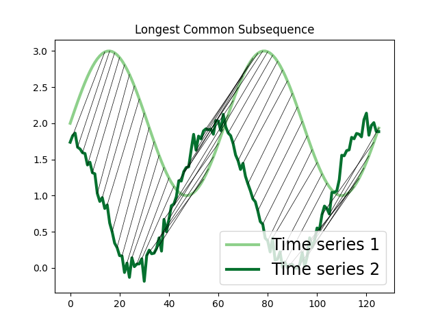
Longest Common Subsequence (LCSS)¶

The Longest Common Subsequence (LCSS) measures the similarity between two time series whose lengths might be different. Since it is formulated based on edit distances, gaps or unmatched regions are permitted and they are penalized with a value proportional to their length. It can be useful to identify similarities between time series whose lengths differ greatly or have noise [1].

In the example below, we compute the LCSS alignment between two time series, one of them with added noise.

import numpy as np
import matplotlib.pyplot as plt
from tssearch.search.query_search import time_series_search
from tssearch.utils.visualisation import plot_alignment

ts1 = np.sin(np.arange(0, 4*np.pi, 0.1))
noise = np.random.normal(0, 0.1, ts1.shape)
ts2 = 1 + np.sin(np.arange(0, 4*np.pi, 0.1) + 2) + noise

ts1 = ts1.reshape(-1, 1)
ts2 = ts2.reshape(-1, 1)

dict_distances = {
    "elastic": {"Longest Common Subsequence": {
        "multivariate": "yes",
        "description": "",
        "function": "lcss",
        "parameters": {"eps": 1, "report": "distance"},
        "use": "yes"}
    }
}

result = time_series_search(dict_distances, ts1, ts2, output=("number", 1))

plt.figure()
plt.title("Longest Common Subsequence")
plot_alignment(ts1, ts2, result["Longest Common Subsequence"]["path"][0])

Time Warp Edit Distance (TWED)¶

Time warp edit distance (TWED) uses sequences’ samples indexes/timestamps difference to linearly penalize the matching of samples for which indexes/timestamps values are too far and to favor the matching samples for which indexes/timestamps values are closed. Contrarily to other elastic measures, TWED entails a time shift tolerance controlled by the stiffness parameter of the measure. Moreover, it involves a second parameter defining a constant penalty for insert or delete operations. If stiffness > 0, TWED is a distance (i.e., verifies the triangle inequality) in both space and time [2].

TWED has been used in time series classification assessing classification performance while varying TWED input parameters [2], [3]. In the example, we calculate TWED between two time series varying its parameters.

import numpy as np
import pandas as pd
import seaborn as sns
import matplotlib.pyplot as plt
from tssearch.distances.compute_distance import time_series_distance

# generates signals
freq = 2
amp = 2
time = np.linspace(0, 2, 1000)
ts1 = amp * np.sin(2 * np.pi * freq * time)
ts2 = amp * np.sin(6 * np.pi * freq * time)[::50]

# visualize original and downsampled sequence
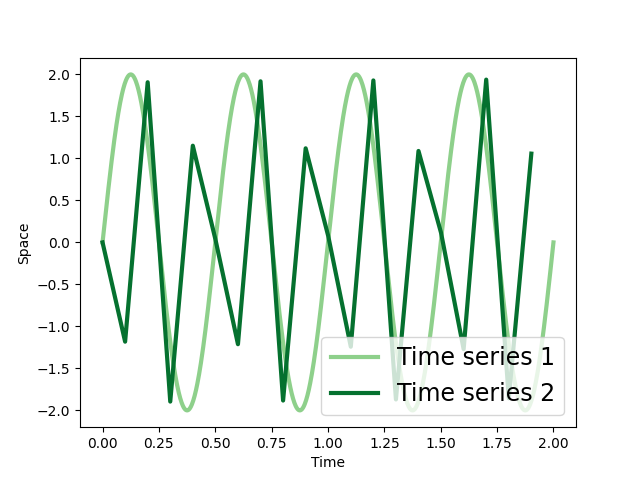
plt.figure()
plt.plot(time, ts1, color=sns.color_palette("Greens")[2], label="Time series 1", lw=3.)
plt.plot(time[::50], ts2, color=sns.color_palette("Greens")[5], label="Time series 2",  lw=3.)
plt.ylabel('Space')
plt.xlabel('Time')
plt.legend(fontsize=17, loc="lower right")

stiffness = [1e-5, 1e-4, 1e-3, 1e-2, 1e-1, 1]
penalty = [0, .25, .5, .75, 1.0]

distance = list()
for s in stiffness:
    for p in penalty:
        # calculate distances
        dict_distances = {
                "elastic": {"Time Warp Edit Distance": {"multivariate": "no",
                                                        "description": "",
                                                        "function": "twed",
                                                        "parameters": {"nu": s, "lmbda": p, "p": 2, "time": "true"},
                                                        "use": "yes"}}}

        distance.append({'stiffness': s,
                         'penalty': p,
                         'distance': time_series_distance(dict_distances,
                                                          ts1, ts2,
                                                          time, time[::50]).values[0][0]})

df = pd.DataFrame(distance)
df_pivot = df.pivot("stiffness", "penalty", "distance")

plt.figure()
sns.heatmap(df_pivot, annot=True, cbar_kws={'label': "TWED"}, cmap="viridis")

[1]	Vlachos, G. Kollios and D. Gunopulos, “Discovering similar multidimensional trajectories,” Proceedings 18th International Conference on Data Engineering, 2002, pp. 673-684, doi: 10.1109/ICDE.2002.994784.

[2]	(1, 2) Marteau, “Time Warp Edit Distance with Stiffness Adjustment for Time Series Matching,” in IEEE Transactions on Pattern Analysis and Machine Intelligence, vol. 31, no. 2, pp. 306-318, Feb. 2009, doi: 10.1109/TPAMI.2008.76.

[3]	Joan Serrà, Josep Ll. Arcos, An empirical evaluation of similarity measures for time series classification, Knowledge-Based Systems, Volume 67, 2014, Pages 305-314, ISSN 0950-7051, https://doi.org/10.1016/j.knosys.2014.04.035.